Agentic Systems as Graphs

Before you start coding a single LLM call for a new agent or harness, you have to answer a much more basic question: what is this agent actually supposed to do, in what order, and under what conditions? It's easy to skip past the business logic, and let an LLM can improvise its way through a fuzzy plan well enough to look like it's working.

During the 60s and 70s computer scientists developed an approach, known as 'structured programming', with the goal of engineering systems in a structured way, with no untraceable or unreproducible steps in the logic. All to prevent that is works only "well enough to look like it's working".

Defining an agent's business logic first — as an explicit graph of steps, decisions, and loops — is what makes the difference between designing a system you can start to evaluate and debug next, and just prompt something and hope for the best. To see why graphs are the right tool to structure our thinking around htis topic, it's worth going back sixty years, to the moment computer science first had to solve exactly these same problem for ordinary computer code.

The Böhm–Jacopini Theorem

In the late 1950s (before modern programming) computer code were still written with goto statements all over the place; a jump to another labeled point in the code. This wasn't a niche practice. It was necessary because a processor understands only very basic operations, like additions, comparisons of numbers, and "jump to this memory address".

FORTRAN, the dominant scientific language of the late 1950s, had no if/else statements or for/while loops yet. The conditional was the arithmetic (IF (X) 10, 20, 30), which evaluated an expression (X), followed by a GOTO jump to one of three line numbers that followed the expression, depending on whether the result was negative, zero, or positive. Loops were built with a numbered DO plus a GOTO back to that line to repeat. COBOL, released around the same time, used GO TO paragraph names to hop between named blocks of code.

It worked, but it was chaos when trying to read computer code. You had to trace line numbers and labels across pages to understand what the program did, and which lines it would read in what order. The control flow could leap anywhere, so reading a program meant mentally tracing jumps scattered across pages, with no guarantee any block of code ran once, always, or a fixed number of times before execution moved on.

In 1966, Corrado Böhm and Giuseppe Jacopini proved something surprising: none of that arbitrary jumping is actually necessary. Any computable function. No matter how tangled the original flowchart is, it can always be rewritten using only three control structures:

• Sequence — do A, then B, then C
• Selection — choose a path based on a condition (if/else)
• Iteration — repeat a block while some condition holds (while/for)

That's it. These tree primitive functions are enough to express any program.

Control-Flow Graphs

To see why Böhm and Jacopini's result matters, it helps to have a way of drawing a program's control flow rather than just reading it. That's a control-flow graph (CFG): a directed graph where the nodes are straight-line chunks of code called basic blocks — sequences of instructions with no jumps in or out except at the very start and end, and the edges are the possible jumps between them.

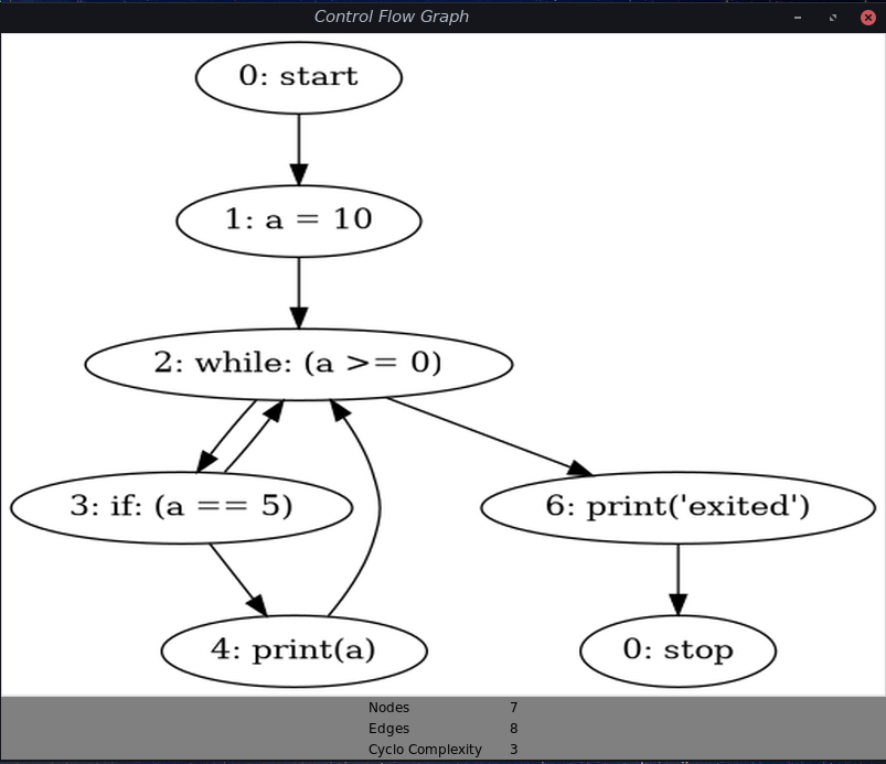
Böhm and Jacopini's proved that any CFG, no matter how tangled, can be rewritten into one built only from sequence, selection, and iteration, without changing the program. A CFG built purely from those three primitives is called reducible. Every loop in a reducible graph has exactly one entry point into a loop. Meaning any path into the loop has to pass through the single header block first.

A goto statement allows us to jump into the middle of a loop from outside, creating a loop with two separate entry points. This is an irreducible graph, one that no amount of relabeling can turn into clean if/while nesting. But we can create a reducible graph, that contains the exact same logic.

This reducible graph block-based approach to structure code in terms of control flows became increasingly popular during the 70s. It was referred to as Structured Programming. Dijkstra's 1968 letter on Go To Statement Considered Harmful lead a lot to its increasing popularity, and in later programming languages the goto statement has no longer been included.

Agentic Systems as Graphs

Fast forward to today. An agentic application — a system where an LLM plans, calls tools, evaluates results, and decides what to do next — that is following some kind of business logic, can have the business logic be described as a graph. Each node in such a graph is a unit of work: an LLM call, a tool invocation, a retrieval step, a human checkpoint.

Each edge is a transition: "after this, do that". Loops allow an agent to retry a failed tool call, refine a draft until it passes a quality check, or loops through a "think, act, observe" cycle and returns to an earlier node.

Just as any program reduces to sequence, selection, and iteration, any graph for an agentic process reduces to four primitive operations: chain, branch, loop, and nest.

1. Chain — sequence A → B → C Nodes execute one after another, output feeding into the next. The default pipeline: no decisions, no repetition.

2. Branch — selection

      → B
A →
      → C

Given a condition, a router, or a classifier, execution splits down different paths. This covers both conditional routing (pick exactly one path, like if/else) and parallel fan-out (run several paths at once and merge the results later).

3. Loop — iteration A → B → (back to A, until condition) A back-edge that lets a node or subgraph re-execute until some exit condition is met. This is what makes retries, self-refinement, and "keep working until the task is done" possible.

Multi-Agentic Systems as Graphs

4. Nest — composition A single node in the outer graph is itself a complete graph — its own chain, branches, and loops — collapsed into a black box. This is the primitive Böhm–Jacopini didn't need to worry about but that agentic systems can't do without: it's what lets a multi-step subprocess be treated as one node in a larger workflow, and lets that subprocess contain its own internal complexity.

Why This Is the Right Minimal Set

The claim is that these four operations are closed and sufficient — every higher-level agentic pattern you've heard of reduces to some composition of them:

• Map-reduce = branch (fan-out across items) + chain (merge results)
• Supervisor–worker = nest (workers as subgraphs) + branch (routing to the right worker) + loop (re-delegate on failure)
• Retry-with-backoff = loop with a conditional exit
• Human-in-the-loop approval = branch that includes a "wait for external input" node

This is the same move Böhm and Jacopini made, one level up. Their theorem gave structured programming a minimal, provably sufficient vocabulary for describing control flow inside a single function. Chain/branch/loop/nest gives agentic system design the same thing — a minimal vocabulary for describing control flow across a graph of LLM calls, tools, and subprocesses, without needing to invent new primitives every time a new agent pattern becomes fashionable.

The practical payoff is the same too. Just as structured programming made code easier to read, debug, and prove correct by ruling out arbitrary jumps, describing agents as compositions of chain/branch/loop/nest makes agentic systems easier to reason about, test, and compose — instead of a tangle of ad hoc control logic that only the person who wrote it can follow.